Grace Hopper developed the first compiler for a computer programming language.
Assignment 2 - Analyzing Branch Predictors
- Assignment 2 - Analyzing Branch Predictors
- Github clone link
- Goals
- Champsim Simulator
- 450/750 Students
- Report preparation
- Check yourself
- 1. Static approaches Q1 and Q2
- 2. Bimodal predictor
- Q3. Bimodal table size $2^8, 2^{10}, 2^{12}, 2^{16}, 2^{20}, 2^{24}$ vs accuracy. On the y-axis, plot “accuracy” (larger is better)
- Q4. Pareto optimality: Given a large enough predictor, what is the best accuracy obtainable by the bimodal predictor?
- Q5. How large must the predictor be to improve accuracy by 2x compared to the better of
always takenandalways not taken(cutting misprediction rate in half)? Give the predictor size both in terms of number of counters as well as bytes. - Q6. What is the smallest predictor table size which is within 3%, 5%, 10% accuracy difference of the $2^{24}$ size.
- 450 Students
- Global predictor
- Q7. Global table size $2^{12}, 2^{16}, 2^{20}, 2^{24}$ vs accuracy. Keep the number of PC bits fixed to 10 and vary the GH bits to increase the table size. Plot accuracy.
- Q8. Global table size $2^{12}$, $2^{16}$, $2^{20}, 2^{24}$ vs accuracy. Keep the number of GH bits fixed to 10 and vary the PC bits to increase the table size. Plot accuracy. Which size performed best?
- Q9. For predictor $2^{24}$ what is the accuracy obtained when GH = 10 bits?
- Q10. For the same table size. ($2^{12}$, $2^{16}$, $2^{20}$, $2^{24}$) which branch predictor performed better; bimodal or global?
- Q11. Explain why global maybe sometimes more accurate then bimodal. Explain why bimodal may sometimes be more accurate than global?
- Local predictor
- Q12. Vary table 2 size ($2^{12}$, $2^{16}$, $2^{20}$, $2^{24}$) and keep the number of PC bits fixed to 10 and vary the LH bits to increase the table size. Plot the accuracy for different configurations.
- Q13. Fix table 2 size to $2^{16}$ i.e., number of LH bits = 16. Vary table 1 size from $2^{6}$ to $2^{12}$ in powers of 2. Plot accuracy for different configurations.
- Tournament predictor (Optional)
- Q14. (Optional). How does the tournament predictor’s accuracy compare to bimodal, local, and global? Is the tournament predictor successful in meeting its goal? Try the following configurations (bimodal=$2^{12}$, local=$2^{12}$, global = $2^{12}$, tournament = $3 \times 2^{12}$). For local and global predictors, use PC and LH bits used in previous questions.
- Q15 (Optional). Does the tournament predictor improve the overall peak (best-case) accuracy? If so, why? If not, what are the benefits of the tournament predictor?
- Fairer Size for Tournament Predictor
- Q16 (Optional). Compare the old and new tournament predictor data. What was the impact of moving to the smaller (fairer) table sizes?
- Q17 (Optional). Once adjusted to be a fair-size comparison, does the tournament predictor succeed in its goal of outperforming both predictors compared to global $2^n$ or local (Table 1: 256 entries, each entry n bits, Table 2: $2^n$) ?
- Global predictor
- 750 Students
- TAGE predictor
- Q18. Plot the accuracy of three TAGE configurations against the bimodal predictor.
- Q19. In configuration 2 change T1-T7 size to 512 entries. Increase T8,T9 to 4K entries. Does accuracy improve or not?
- Q20. Create a histogram for worst-performing branches. What is the accuracy on the top-20 branches with worse-accuracy?
- TAGE predictor
- Grading criteria
- Acknowledgments
Github clone link
Goals
In this assignment you will explore the effectiveness of branch direction prediction (taken vs not taken) on an actual program. Your task is to use the spec 2017 benchmarks traces to evaluate the effectiveness of a few real-life branch prediction schemes. The objective is to compare different branch prediction algorithms in a common framework. Predictors will be evaluated for conditional branches.
Champsim Simulator
ChampSim is a trace-based function-first simulator used for microarchitecture studies.
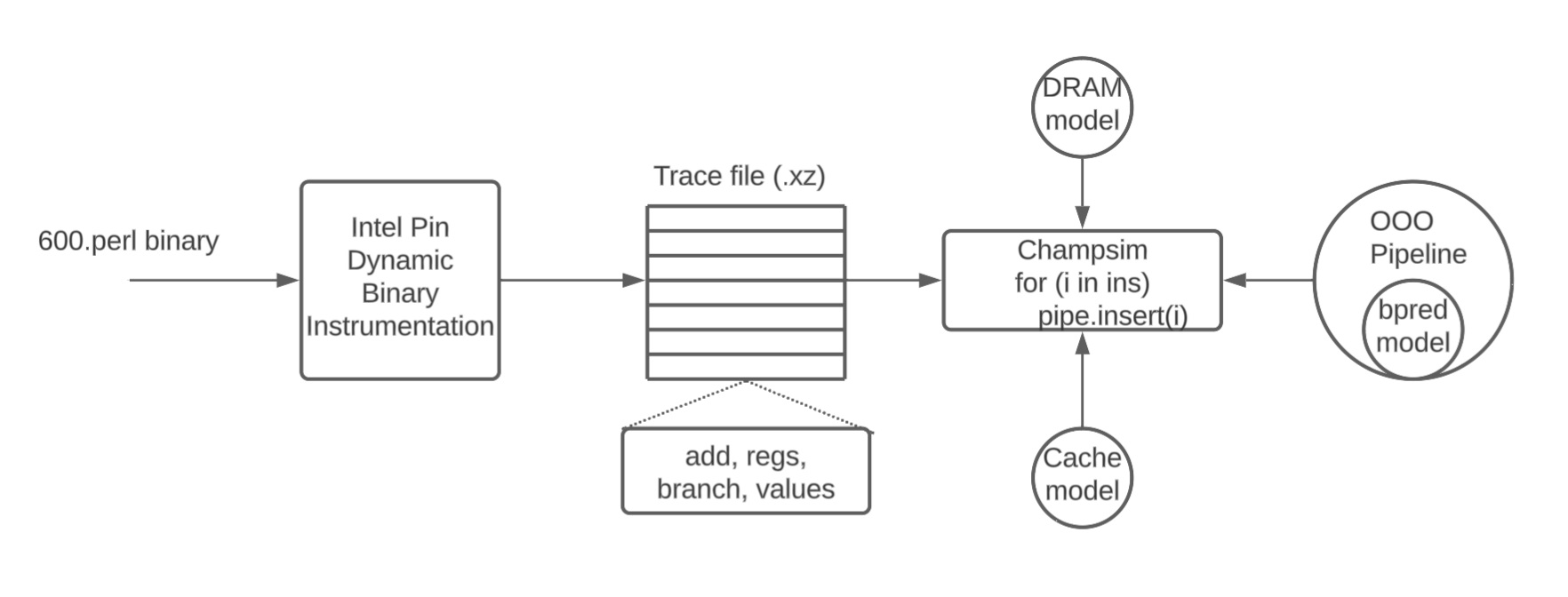
ChampSim takes five parameters: Branch predictor, L1D prefetcher, L2C prefetcher, LLC replacement policy, and the number of cores (We will only be conducting single core). For example,
cd $REPO
#  builds a single-core processor with bimodal branch predictor, no L1/L2 data prefetchers, and the baseline LRU replacement policy for the LLC
 ./build_champsim.sh bimodal no no no no lru 1

# Link to spec 2017 traces
export TRACE_DIR=/data/dpc3_traces/
./run_champsim.sh bimodal-no-no-no-no-lru-1core 1 10 600.perlbench_s-210B.champsimtrace.xz
# This will take about 1-2minutes
# When debugging try at most 1 million instruction trace before moving onto longer traces.
# Result file will be "results_${N_SIM}M" as a form of "${TRACE}-${BINARY}-${OPTION}.txt".
| Param | Description |
|---|---|
| 1 | number of instructions for warmup (1 million) |
| 10 | number of instructions for detailed simulation (10 million) |
Results file
$ cat results_10M/600.perlbench_s-210B.champsimtrace.xz-bimodal-no-no-no-no-lru-1core.txt

CPU 0 Bimodal branch predictor

Warmup complete CPU 0 instructions: 1000001 cycles: 401571 (Simulation time: 0 hr 0 min 4 sec)

Heartbeat CPU 0 instructions: 10000000 cycles: 7410810 heartbeat IPC: 1.34938 cumulative IPC: 1.28402 (Simulation time : 0 hr 0 min 32 sec)

CPU 0 Branch Prediction Accuracy: 97.771% MPKI: 3.658 Average ROB Occupancy at Mispredict: 83.3361

Branch types
NOT_BRANCH: 8358572 83.5857%
BRANCH_DIRECT_JUMP: 200075 2.00075%
BRANCH_INDIRECT: 64447 0.64447%
BRANCH_CONDITIONAL: 1196085 11.9609%
BRANCH_DIRECT_CALL: 83309 0.83309%
BRANCH_INDIRECT_CALL: 6936 0.06936%

Branch misprediction for individual branch types
BRANCH_DIRECT_JUMP: 245 0.122454%
BRANCH_INDIRECT: 20 0.0310333%
BRANCH_CONDITIONAL: 45785 3.82792%                    # <-- We use misprediction rate conditional branches only
BRANCH_DIRECT_CALL: 141 0.169249%
BRANCH_INDIRECT_CALL: 10 0.144175%
BRANCH_RETURN: 121 0.134078%
BRANCH_OTHER: 0 -nan%
Add your own branch predictor
cp branch/branch_predictor.cc branch/mybranch.bpred
Each branch predictor needs to atleast implement 3 handlers
// bimodal.pred
// Initialize the state of your branch predictor
void O3_CPU::initialize_branch_predictor()
{
  // Initialize values to not taken
}

// Invoked on conditional branch by the pipeline
uint8_t O3_CPU::predict_branch(uint64_t ip)
{
  // if return 1; branch is taken
  // if return 0; branch is not-taken
}

// A useful C++ std function is std::clamp.
// Update/Repair
void O3_CPU::last_branch_result(uint64_t ip, uint8_t taken)
{
  // Change the counter values.
  // Deallocate/allocate entries if required.
}
# Everytime you change the pred file. Remember to rebuild
 ./build_champsim.sh mybranch no no no no lru 1
450/750 Students
Report will be prepared in markdown. For each of the questions below experiment with 10 million instructions from the benchmarks listed.
- 450 students can do in groups of up to two students.
- Only one person has to create the repository. You can add the other person in settings after you create the repository.
Report preparation
- Reports will be prepared in markdown (REPORT.md in the root of your repository)
- You can export markdown to pdf using markdown vistual studio to pdf
- Report files will be named REPORT.md and REPORT.pdf
- REPORT.pdf should be submitted on Canvas.
We will be using the following traces to experiment with different branch predictors and configurations:
- 600.perlbench_s-210B.champsimtrace.xz
- 602.gcc_s-734B.champsimtrace.xz
- 625.x264_s-18B.champsimtrace.xz
- 641.leela_s-800B.champsimtrace.xz
- 648.exchange2_s-1699B.champsimtrace.xz
Check yourself
Do not proceed without comprehending these bullets. Refresh the material below and fix an instructor OH if you are not able to answer any of these questions.
- Do you know how to mask and extract bits from address ? If not familiar, watch 295 video
- Do you know what is a direct mapped cache ?
- If a hardware table is indexed by a K-bit index, how many entries does the table have ?
- Do you know how to implement a saturation counter (e.g., 2-bit up/down saturating counter)?
- Do you know how to implement a state machine like the one on Slide 7 of Week2’s Lecture Notes?
- Why do we skip the least significant two bits in the branch PC when indexing into a branch prediction table ?
- What is the difference between global branch history and local branch history ?
- Why does aliasing happen in branch predictors ?
- How do you implement an N bit shift buffer ? C++ rotate
1. Static approaches Q1 and Q2
Before looking at dynamic branch prediction, we are going to implement simple static branch prediction policies of
- always predict taken
taken.pred -
always predict not taken
not-taken.pred. (You can implement these two prediction policies by following the instructions under Add your own branch predictor section) - calculate the mis-prediction rate (that is, the percentage of conditional branches that were mis-predicted) for these two simple schemes. To answer the following questions, plot the mis-prediction statistics for all the benchmarks using either bar or line charts.
Q1. Which of these two policies is more accurate (has fewer mis-predictions)?
Q2. Based on common programming idioms, what might explain the above result?
You can use excel or matplotlib to generate the plots: see here for line plots:
Grouped bar charts in Matplotlib Simple plot tutorial using Matplotlib
2. Bimodal predictor
The simplest dynamic branch direction predictor is an array of $2^n$ two-bit saturating counters. Each counter includes one of four values: strongly taken (T), weakly taken (t), weakly not taken (n), and strongly not taken (N).
This has already been provided to you at branch/bimodal.pred
- Saturating counter
- 16384 entries
- 2 bit counter
- counter value
init = 0
Prediction: To make a prediction, the predictor selects a counter from the table using using the lower-order n bits of the instruction’s address (its program counter value). The direction prediction is made based on the value of the counter.
Training: After each branch (correctly predicted or not), the hardware increments or decrements the corresponding counter to bias the counter toward the actual branch outcome (the outcome given in the trace file). As these are two bit saturating counters, decrementing a minimum counter or incrementing a maxed out counter should have no impact.
Q3. Bimodal table size $2^8, 2^{10}, 2^{12}, 2^{16}, 2^{20}, 2^{24}$ vs accuracy. On the y-axis, plot “accuracy” (larger is better)
Q4. Pareto optimality: Given a large enough predictor, what is the best accuracy obtainable by the bimodal predictor?
Q5. How large must the predictor be to improve accuracy by 2x compared to the better of always taken and always not taken (cutting misprediction rate in half)? Give the predictor size both in terms of number of counters as well as bytes.
Q6. What is the smallest predictor table size which is within 3%, 5%, 10% accuracy difference of the $2^{24}$ size.
450 Students
Bimodal predictor maintain a 2-bit saturating counter for each entry (or use 10 branch PC bits to index into one of 1024 counters) – captures the recent ``common case’’ for each branch. Here we try to take advantage of additional information. Intuition 0 (Not taken), 1 (taken)
- If a branch recently went NTTTT, expect N; if it recently went TTTNT, expect T; can we have a separate counter for each case?
You task is to build correlating predictors or two-level branch predictor. We will build two kinds. Those that take advantage of global history and those that take advantage of local history and then conduct a tournament between the two.
Instead of maintaining a counter for each branch to capture the common case
- Maintain a counter for each branch and surrounding pattern
- If the surrounding pattern belongs to the branch being predicted, the predictor is referred to as a local predictor
- If the surrounding pattern includes neighboring branches, the predictor is referred to as a global predictor
Global predictor
Instead of using only the PC to predict if a branch is taken or not, the global predictor uses the last N branches. For instance, if the last N branches were TNTNTN, you might predict the next branch would be taken.
- The global history register consists of GH bits
- You obtain the bottom PC bits from instruction pointer and concatenate the two (PC+GH bits).
- This is capable of addressing a table with $2^{PC+GH}$ entries.
- Each entry is a 2 bit saturating counter.
The rest of the implementation is similar.
- increment entry if branch T
- decrement entry if branch N
- refer to entry for prediction.
Q7. Global table size $2^{12}, 2^{16}, 2^{20}, 2^{24}$ vs accuracy. Keep the number of PC bits fixed to 10 and vary the GH bits to increase the table size. Plot accuracy.
Q8. Global table size $2^{12}$, $2^{16}$, $2^{20}, 2^{24}$ vs accuracy. Keep the number of GH bits fixed to 10 and vary the PC bits to increase the table size. Plot accuracy. Which size performed best?
Q9. For predictor $2^{24}$ what is the accuracy obtained when GH = 10 bits?
Q10. For the same table size. ($2^{12}$, $2^{16}$, $2^{20}$, $2^{24}$) which branch predictor performed better; bimodal or global?
Q11. Explain why global maybe sometimes more accurate then bimodal. Explain why bimodal may sometimes be more accurate than global?
Local predictor
A two-level predictor that only keeps local histories at the first level. There are two tables.
-
Table 1: Local history table. Indexed by PC bits. Maintains LH bits of local histories for each PC. The size of the local table is $2^{PC}$. Each entry tracks the most recent $LH$ taken/not-taken of the particular tag.
-
Table 2: Indexed based on history from the first table. Total entries = $2^{LH}$. Each entry is a 2-bit counter.
Check yourself What is the total size of the local table ?
Q12. Vary table 2 size ($2^{12}$, $2^{16}$, $2^{20}$, $2^{24}$) and keep the number of PC bits fixed to 10 and vary the LH bits to increase the table size. Plot the accuracy for different configurations.
Q13. Fix table 2 size to $2^{16}$ i.e., number of LH bits = 16. Vary table 1 size from $2^{6}$ to $2^{12}$ in powers of 2. Plot accuracy for different configurations.
Tournament predictor (Optional)
This part of the homework is optional. Extra credit will be given to students who complete this part.
From the previous data, you can see that neither global or local is always best. To remedy this situation, we can use a hybrid predictor that tries to capture the best of both style of predicts. A tournament predictor consists of three tables. The first and second tables are just normal global and local predictors. The third table is a chooser table that predicts whether the global or local predictor will be more accurate.
The basic idea is that some branches do better with a global predictor and some do better with a local predictor. So, the chooser is a table of two-bit saturating counters indexed by the low-order bits of the PC that determines which of the other two table’s prediction to return. For the choose, the two-bit counter encodes: strongly prefer global (B), weakly prefer global (b), weakly prefer local (g), and strong prefer local (G).
Let’s compare the tournament predictor’s accuracy versus the data from its two constituent predictors (using the data from the previous question). For now, let’s compare a $2^n$ counter local (or global) versus a tournament predictor with three $2^n$ counter tables. (We’ll make the comparison more fair in terms of a ``same number of bits’’ comparison in a moment.) As above for the local predictor, the local component of the tournament predictor should use a history length equal to the number of index bits (log of the table size). The graph will have three lines total.
Q14. (Optional). How does the tournament predictor’s accuracy compare to bimodal, local, and global? Is the tournament predictor successful in meeting its goal? Try the following configurations (bimodal=$2^{12}$, local=$2^{12}$, global = $2^{12}$, tournament = $3 \times 2^{12}$). For local and global predictors, use PC and LH bits used in previous questions.
Q15 (Optional). Does the tournament predictor improve the overall peak (best-case) accuracy? If so, why? If not, what are the benefits of the tournament predictor?
Fairer Size for Tournament Predictor
In the previous question, the tournament predictor was given the unfair advantage of having three times the storage. In this question, run another set of experimental data in which all the predictors at the same location on the x-axis have the same storage capacity. To do this, compare let total entries be $2^n$ for tournament predictor with the following three table sizes:
- Global table size : $2^{n-1}$
- Local table 2 size : $2^{n-2}$ Local table 1 size : $2^8$ entries, n-2 bits per entry.
- Chooser table size : $2^{n-2}$ 2 bit counters.
Total $\simeq$ a $2^n$ global or local. Vary n = $12,16,20,24$
Q16 (Optional). Compare the old and new tournament predictor data. What was the impact of moving to the smaller (fairer) table sizes?
Q17 (Optional). Once adjusted to be a fair-size comparison, does the tournament predictor succeed in its goal of outperforming both predictors compared to global $2^n$ or local (Table 1: 256 entries, each entry n bits, Table 2: $2^n$) ?
750 Students
This part of the homework is only for 750 students. You will implement a TAGE branch predictor.
TAGE predictor
You will implement a variant of one of the best branch-predictors of all time and the winner of three consecutive branch predictor competitions, TAGE ref1 TAGE ref2 Figure illustrates a TAGE predictor.
The TAGE predictor features a base predictor T0 in charge of
providing a basic prediction and a set of (partially) tagged predictors $T_i$ (i=1..M). These tagged predictor components $T_i$, are indexed using different history lengths that form a geometric series, i.e, $L(i) = \alpha^{i-1} * L(1) + 0.5$. The the base predictor $L_0$ will be a simple PC-indexed 2-bit counter bimodal table. Note that essentially we maintain a single global history table with maximal width and simply pick the relevant shorter history where required. An entry in a tagged component consists of a signed counter ctr which sign provides the prediction, a (partial) tag and an unsigned useful counter u. u is a 2-bit counter and ctr is a 2-bit counter.
Similar to a tournament predictor, multiple tables provide a prediction. The $T_{pred}$ provider is the matching table with the longest history. The alternate prediction $T_{alt}$ is the prediction that would have occurred if there had been a miss on the provider component. If there is no matching tag component altpred is the $T_0$ (bimodal prediction).
| Rule 1: Prediction. | Find Table $T_{pred}$ with the longest history. If ctr is weak or u is 0 then $T_{alt}$ provides prediction |
| Rule 2: ctr | On a correct prediction, ctr of both $T_{Pred}$ is updated. If incorrect its decremented. |
| Rule 3: useful | The useful counter u of the $T_{pred}$ table is updated when the $T_{alt}$ $\neq$ $T_{pred}$ and prediction is correct. The useful counter u is also used as an age counter and is gracefully reset every 512K branches. useful exists only in Tage table |
| Rule 4: Allocation entries | On mispredictions at most one entry is allocated. If the provider component $T_{pred}$ is not the longest, we try to allocate an entry on a predictor component $T_k$ ($pred \leq k \leq M$). The allocation process is described below. |
- We search for entries starting from $T_{pred}$, with $T_{pred+1}$ with probability 1/2, $T_{pred+2}$, with probability 1/4 and $T_{pred+3}$ with probability 1/4. An allocated entry is initialized with the prediction counter set to weak correct. Counter u is initialized to 0 (i.e., strong not useful). If unable to find a free entry the u counter of $T_{pred}$ is decremented.
Finally, the hash and tag functions. The hash function determines which entry in the table does a particular branch gets allocated in. We use an xor function to calculate the index. Why XOR function. We split the PC and global history of the table into index-wide segments and xor them with each other. We similarly calculate the tags, however the width of the segments depend on the number of tag width.
Q18. Plot the accuracy of three TAGE configurations against the bimodal predictor.
You can compare your results to the championship winning TAGE here. Note that the championship winner uses loop predictors and other patterns. It also uses different hash and index functions so your results may not match completely. At least you should be in the ballpark.
Run the following benchmarks. You will fastforward for 1 million instructions and run for 10 million instructions.
- 602.gcc_s-734B.champsimtrace.xz
- 603.bwaves_s-3699B.champsimtrace.xz
- 607.cactuBSSN_s-2421B.champsimtrace.xz
- 621.wrf_s-575B.champsimtrace.xz
- 623.xalancbmk_s-700B.champsimtrace.xz
- 625.x264_s-18B.champsimtrace.xz
- 627.cam4_s-573B.champsimtrace.xz
- 628.pop2_s-17B.champsimtrace.xz
- 631.deepsjeng_s-928B.champsimtrace.xz
- 641.leela_s-800B.champsimtrace.xz
- 648.exchange2_s-1699B.champsimtrace.xz
- 649.fotonik3d_s-1176B.champsimtrace.xz
- 654.roms_s-842B.champsimtrace.xz
- 657.xz_s-3167B.champsimtrace.xz
Configuration 1: ~70K bits. 4 tables + 1 bimodal TAGE.
| T1,T2 | T3,T4 | |
|---|---|---|
| History length | 4 6 | 10 16 |
| Table entries | 1K | 2K |
| Tag width | 7 | 8 |
| Storage budget | 11K | 24K |
Configuration 2: ~171K bits. 9 tables + 1 bimodal TAGE.
| T1,T2 | T3,T4 | T5 | T6 | T7 | T8,T9 | |
|---|---|---|---|---|---|---|
| History length | 4 6 | 10 16 | 25 | 40 | 64 | 101,160 |
| Table entries | 1K | 2K | 2K | 2K | 1K | 1K |
| Tag width | 7 | 8 | 9 | 10 | 11 | 12 |
| Storage budget | 11K | 24K | 26K | 28K | 15K | 16K |
Configuration 3: ~204.5K bits. 12 tables + 1 bimodal TAGE.
| T1,T2 | T3,T4 | T5 | T6 | T7 | T8,T9 | T10 | T11 | T12 | |
|---|---|---|---|---|---|---|---|---|---|
| History length | 4 6 | 10 16 | 25 | 40 | 64 | 101,160 | 254 | 403 | 640 |
| Table entries | 1K | 2K | 2K | 2K | 1K | 1K | 1K | 0.5K | 0.5K |
| Tag width | 7 | 8 | 9 | 10 | 11 | 12 | 13 | 14 | 15 |
| Storage budget | 11K | 24K | 26K | 28K | 15K | 16K | 17K | 9K | 9.5K |
Use the same base bi-modal predictor in all configs: 16K entries, 2 bit counter.
Q19. In configuration 2 change T1-T7 size to 512 entries. Increase T8,T9 to 4K entries. Does accuracy improve or not?
Q20. Create a histogram for worst-performing branches. What is the accuracy on the top-20 branches with worse-accuracy?
Grading criteria
- Answer the questions in REPORT.md and those specified here
- If you do not include (or refer to) plots for each question it will simply be zeroed out.
WARNING: Do not simply include a data dump - The total assignment is worth a 150 points equally split among mandatory questions. The extra credit part is worth 20% more.
- Commit the report to the repo in .md and .pdf formats. Submit the pdf also on canvas (for groups, each member needs to submit the same pdf copy on canvas)
- You also need to include a README in your repo with instructions on which commands to run to generate results and plots.
PDF Submission Canvas
Acknowledgments
This assignment has been modified by the CMPT 450/750 instructors.