Grace Hopper developed the first compiler for a computer programming language.
Assignment 4 - Tiled and Sparse Matrix Multiplication
- Assignment 4 - Tiled and Sparse Matrix Multiplication
- Github clone link
- Dense Matrix Dense Matrix Tiled Multiplication (GEMM)
- Testbench
- Report preparation
- Instructions
- Task 1: Implement the following three dataflows and compare performance
- Q1 : What is the best dataflow for small matrices? Why?
- Q2 : What is the best dataflow for medium matrices? Why?
- Q3 : What is the best dataflow for large matrices? Why?
- Q4: If you transposed the matrices to store them in their preferred format prior to the GEMM operation, how would that affect the performance? Plot as stacked bars with transpose included separately in performance for different dataflows.
- Q5: Can you improve the performance of the transpose operation itself (Hint: Use blocking and parallelize the transpose of each block using OpenMP) Investigate the performance for tile sizes from 4x4, 8x8, 16x16, 32x32 and plot the performance.
- Task 2: Parallelize outer loop - OpenMP or Pthreads
- Q6: What is the improvement in performance of Gustavson’s dataflow? Plot the performance for different number of threads from 1 - 16 (powers of two).
- Q7: What is the improvement in performance of inner product dataflow? Plot the performance for different number of threads from 1 - 16 (powers of two).
- Task 3: Tiling inner loops
- Sparse Matrix - Dense Matrix Multiplication (SpMM)
- Convolutions vs Matrix Multiplication
- Grading
Github clone link
Dense Matrix Dense Matrix Tiled Multiplication (GEMM)
The GEMM (General Matrix-Matrix Multiply) operation multiplies two matrices, $A$ and $B$. These matrices have dimensions $M$×$K$ and $K$×$N$, respectively. The dimension $K$ is shared between both matrices. When we multiply these matrices, the most common method is to use a triple-nested loop to combine their elements appropriately. Implementing GEMM involves iterating over the $M$ and $N$ dimensions and also co-iterating over the shared dimension $K$.
“Co-iteration” is the process of iterating together over the shared dimension $K$ for both matrices during multiplication. Depending on which level of the nested loops we choose to place this co-iteration, we get different dataflows for performing the multiplication:
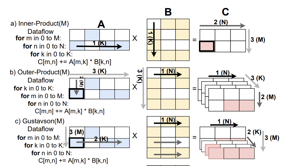
Inner Product (IP): Places the co-iteration at the innermost loop. Think of it as focusing on a single element of the resulting matrix and accumulating its value by iterating over the shared dimension. This method generates a single full sum of each resulting element at a time without merging partial sums.
Outer Product (OP): Puts the co-iteration at the outermost loop. This involves multiplying a single row from $A$ with a single column from $B$ to produce an entire matrix, and then aggregating these matrices to get the final result. This method generates multiple partial sums at a time, requiring merging hardware and potentially increased memory traffic.
Gustavson’s (Gust): Features the co-iteration at the middle loop. This method generates partial sums in the current fiber (i.e., the current row of $A$ and column of $B$) and then aggregates them to get the final result.
Beyond just co-iterating over $K$, we also loop over dimensions $M$ and $N$. The order in which we loop over these independent dimensions $M$ and $N$ can also affect our computation pattern. In fact, for each of the three dataflows (IP, OP, Gustavson’s), changing the loop order for $M$ and $N$ can give us two distinct variants. That’s why we end up with six possible variations.
The importance of choosing one variant over another largely comes down to “data reuse”. In computing, it’s efficient to reuse data that’s already loaded into fast memory (like a cache). By prioritizing the stationarity of a particular dimension (i.e. kept close to the processing elements), we can better reuse data, making computations more efficient. The three different methods are depicted in the figure below. Image Credit
Testbench
- Inputs to use for testing can be copied from the path
/data/a4-inputs. You In all the tasks, you may use the inputs from this repository. You have to test your implementations with inputs of different sizes and densities.
$ cd $REPO
$ cp /data/a4-inputs ./inputs -r
The file naming format is as follows:
- dense: dense_
_ .bin - sparse: sparse_
_ _density _block .bin
You can also generate your own test inputs:
# Create dense matrix of size 4x4
$ python3 bcsr/generate_blocked.py --create-dense 1 -nrows 4 -ncols 4 -output dense_4_4.bin
# Print dense matrix
$ python3 bcsr/generate_blocked.py --print-dense  1 -input dense_4_4.bin
| Files | Description |
|---|---|
| gemm/tiled_gemm.cpp | You will implement the gemm for dense matrices methods in this file. |
| gemm/dense_dense_gemm.py | This is a python interface to invoke the dense gemm methods. |
| bcsr/tiled_spmm.cpp | You will implement the gemm for Sparse-Dense matrices methods in this file. |
| bcsr/bcsr_dense_mm.py | This is a python interface to invoke the Sparse-Dense gemm methods. |
- To run naive matrix multiplication based on inner product:
$ cd $REPO
$ export PYTHONPATH=$PWD/bcsr/:$PYTHONPATH

# Generate a small dense matrix of dimensions 4x4
$ python3 bcsr/generate_blocked.py --create-dense 1 -nrows 4 -ncols 4 -output dense_small.bin
# Print the generated matrix
$ python3 bcsr/generate_blocked.py --print-dense  1 -input dense_small.bin

# Compile the CPP file containing GEMM code
$ g++ -O3 -std=c++11 -shared -o dense_mult.so -fPIC gemm/tiled_gemm.cpp

# Multiply the generated matrix by itself.
$ python3 gemm/dense_dense_mm.py --bin ./dense_mult.so --input_a dense_small.bin --input_b dense_small.bin -o result.bin
- You can modify the python file for testing other methods implemented in tiled_gemm.cpp. You will then need to change the called function from python at line 55 in
dense_dense_mm.py.
Report preparation
- Report files are called
REPORT.mdandREPORT.pdf. REPORT.mdshould contain answers to all the questions and plots in markdown format.- Convert
REPORT.mdtoREPORT.pdf. You can use the VSCode Markdown PDF extension to convert markdown to pdf. - Organize all your plots into a directory called
plots. - Submit your
REPORT.pdfon canvas at https://canvas.sfu.ca/courses/1369/assignments/70679.
Instructions
- For all the timing tasks, you must run the code at least 3 times and report the average to get a more accurate estimate of the performance.
- You should try at least one small, one medium, and one large input for each task unless otherwise specified.
Task 1: Implement the following three dataflows and compare performance
| Dataflow | Static | Tiled | Streamed | A fmt | B preferred fmt | C fmt |
|---|---|---|---|---|---|---|
| MNK Inner Product | C | A | B | Row | Col | Row |
| KMN Outer Product | A | B | C | Column | Row | Row |
| MKN Gustavson’s | A | C | B | Row | Row | Row |
- Implement all three dataflows and compare them with each other for different matrices. For Q1-Q3 assume all matrices are in row major format.
Q1 : What is the best dataflow for small matrices? Why?
Q2 : What is the best dataflow for medium matrices? Why?
Q3 : What is the best dataflow for large matrices? Why?
Q4: If you transposed the matrices to store them in their preferred format prior to the GEMM operation, how would that affect the performance? Plot as stacked bars with transpose included separately in performance for different dataflows.
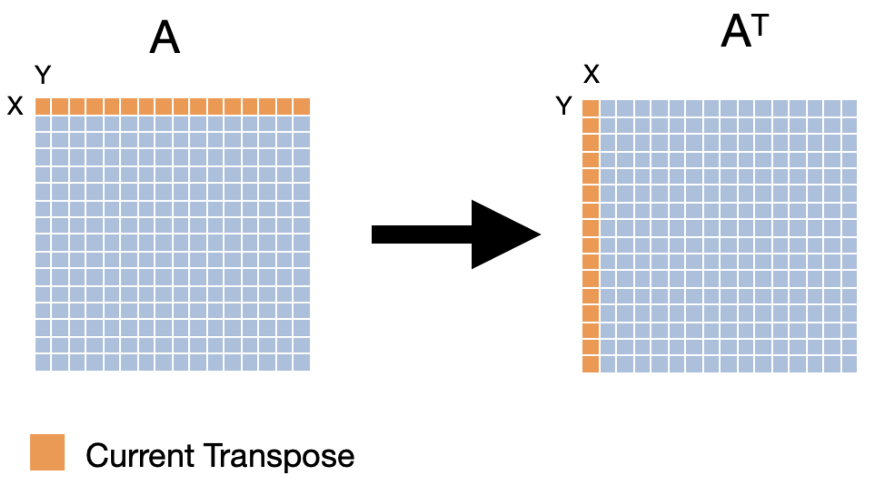
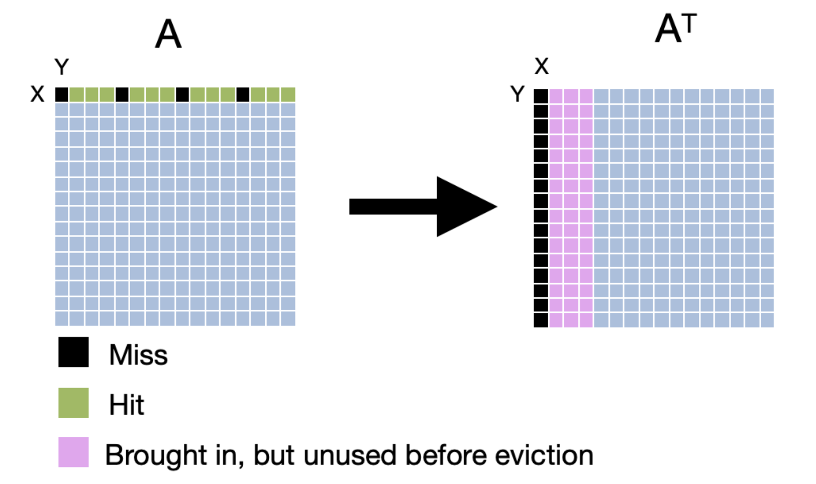
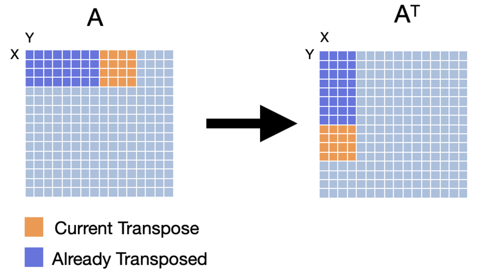
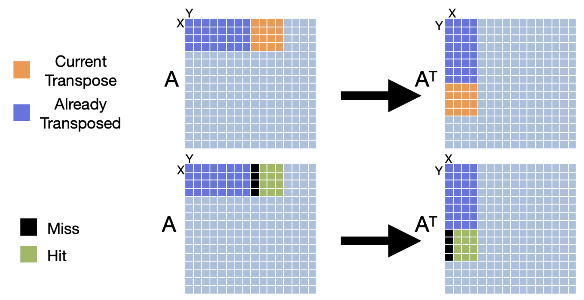
To improve the performance of our transpose, we can use a technique called cache blocking. Cache blocking is a technique that attempts to reduce the cache miss rate by improving the temporal and/or spatial locality of memory accesses. To achieve this, we will transpose the matrix one “block” at a time. We will make sure that the number of bytes within the width of the block can fit into an entire cache line. The following images compares transposition without blocking (base case) and with blocking. It’s worth noting that the effectiveness of tiled matrix transposition depends on factors such as the size of the matrix, cache sizes, and memory access patterns. For example, if the matrix is small enough to fit in the cache, then the tiled approach may not offer any performance benefits. Similarly, if the matrix is already stored in a contiguous memory region, then the tiled approach may not be necessary.
The process of tiled matrix transposition involves the following steps:
- Divide into Tiles: The original matrix is divided into smaller tiles. These tiles are chosen such that they fit well within the cache.
- Transpose Tiles: Each tile is transposed independently. This involves swapping the elements within the tile to their corresponding positions in the transposed matrix.
- Rearrange Tiles: The transposed tiles are rearranged to form the final transposed matrix.
Q5: Can you improve the performance of the transpose operation itself (Hint: Use blocking and parallelize the transpose of each block using OpenMP) Investigate the performance for tile sizes from 4x4, 8x8, 16x16, 32x32 and plot the performance.
Task 2: Parallelize outer loop - OpenMP or Pthreads
In this task, you will parallelize the outer loop of the GEMM operation. The idea is to distribute the rows of the output matrix among the available threads. This distribution can be viewed as decomposing the problem into smaller sub-tasks. Please refer to the OpenMP tutorials below for more details.
Q6: What is the improvement in performance of Gustavson’s dataflow? Plot the performance for different number of threads from 1 - 16 (powers of two).
Q7: What is the improvement in performance of inner product dataflow? Plot the performance for different number of threads from 1 - 16 (powers of two).
Task 3: Tiling inner loops
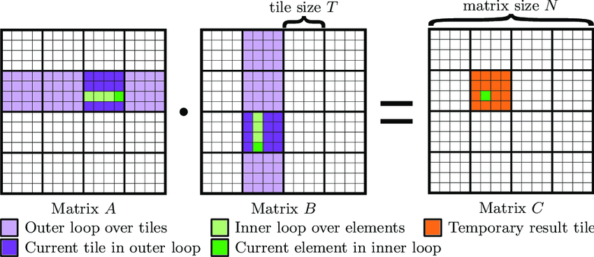
Tiling, also known as blocking, is a common optimization technique used in matrix multiplication, especially in the context of General Matrix Multiply (GEMM) in numerical linear algebra. The idea behind tiling is to improve data locality by dividing matrices into smaller sub-matrices or “tiles”, and then performing the multiplication operation on these smaller chunks. Tiling is one method to make the multiplication more cache-friendly by ensuring that the data being operated on fits inside the fast cache memory and can be reused before it’s evicted.
Modern processors have a memory hierarchy that consists of different types of memory/storage units. This includes registers, different levels of cache (L1, L2, L3, etc.), main memory (RAM), and possibly others. Access time varies greatly between these units; for instance, accessing the L1 cache is much faster than accessing the main memory.
In this task, you will implement tiling for the inner loops of the GEMM operation. The idea is to divide the matrices into smaller tiles and then perform the multiplication on these tiles. The following pseudo-code and figure illustrate the concept of tiling for the inner loops of GEMM. You need to also parallelize the outer loop using either OpenMP or pthreads.
function Tiled_Inner(A, B, C, M, N, K, blockSize):
    for m from 0 to M step blockSize:
        for n from 0 to N step blockSize:
            for k from 0 to K step blockSize:

                // Calculate upper bounds for each block
                mUpper = m + blockSize
                nUpper = n + blockSize
                kUpper = k + blockSize

                for i from m to mUpper:
                    for j from n to nUpper:
                        temp = 0
                        for l from k to kUpper:
                            temp += A[i][l] * B[l][j]
                        C[i][j] += temp
end function
Q8: What is the improvement in performance of Gustavson’s dataflow for tile sizes 4x4, 8x8, 16x16, 32x32? Plot the performance for using different number of threads from 1 - 16 (powers of two).
Sparse Matrix - Dense Matrix Multiplication (SpMM)
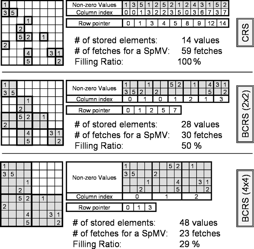
Sparse matrices are matrices that are mostly filled with zero (or another default value) and have only a few non-zero elements. Representing them in the conventional dense format is often inefficient in terms of both memory and computation. That’s where sparse storage formats, such as BSR, come in handy.
Here’s a breakdown of the BSR format. In the BSR format, the sparse matrix is divided into small dense sub-matrices called blocks. These blocks have a fixed size $R \times C$ , where $R$ is the row block size and $C$ is the column block size. These blocks are then stored in a compressed sparse row format.
Use Cases: BSR is particularly efficient when non-zero elements are clustered into small dense blocks. If the matrix exhibits this kind of structure, the BSR format can offer better performance than other formats. Figure illustrates the BCSR format.
BSR format uses three main data arrays:
| Members | Description |
|---|---|
| blockValues | This is a 2D array that stores the dense blocks. It has a shape of (nnz_blocks, R, C), where nnz_blocks is the number of non-zero blocks. |
| Colidx | This is a 1D array of column indices that specify the col ids of nz blocks within a row. |
| RowPtr | Similar to the CSR format, the RowPtr array defines the starting and ending index for each row of blocks in the indices array. |
We have provided a python script for generating and transforming BSR matrices. You can use this script to generate BSR matrices from dense matrices and vice versa. You can also print the generated BSR matrices. The script also supports generating BSR matrices with a specific block size. The following commands illustrate how to use the script:
# Create BCSR matrix. 50% density. Block size : 2
$ python3 bcsr/generate_blocked.py --create-csr 1 -nrows 4 -ncols 4 -density 0.5 -blocksize 2 -output bcsr_half_density.bin

# Print BCSR matrix
$ python3 bcsr/generate_blocked.py --print-csr 1 -input bcsr_half_density.bin

# Convert to block size 4. Input block size is not required. It is encoded in the file.
$ python3 bcsr/generate_blocked.py --transform-bcsr 1 -input bcsr_half_density.bin -blocksize 4 -output bcsr_4.bin

# Convert Dense to BCSR matrix with block size 2.
$ python3 bcsr/generate_blocked.py --transform-dense 1 -input dense_small.bin -blocksize 2 -output bcsr_2.bin
To run testbench
# Make sure the bcsr and dense have compatible columns and rows.  This Python
# script multiplies a Blocked CSR matrix by a dense matrix (in that order), and
# stores the result in result.bin
$ python3 bcsr/bcsr_dense_mm.py -bcsr bcsr.bin -dense dense.bin -o result.bin

# To run the C++ version (you have to implement) in bcsr/tiled_spmm.cpp, run:
$ g++ -shared -o bcsr_mult.so -fPIC bcsr/tiled_spmm.cpp
$ python3 bcsr/bcsr_dense_mm.py -bin bcsr_mult.so -bcsr bcsr.bin -dense dense.bin -o result.bin
Task 1: Implement Gustavson’s dataflow for SpMM.
Let’s break down why Sparse Matrix Multiplication (SpMM) can be more favorable than dense general matrix-matrix multiplication (GEMM) for certain matrices.
- Memory Efficiency When a matrix is sparse (i.e., has a significant number of zeros), storing it in a sparse format (like CSR, CSC, BCSR, etc.) can lead to substantial memory savings. This is crucial when working with large-scale problems where the matrix can be too large to fit in cache if stored densely. In contrast, a dense GEMM operation requires storing every single value in the matrix, including zeros, which can be memory-inefficient for very sparse matrices.
- Computational Efficiency With SpMM we only perform multiplications and additions for non-zero elements, which reduces the number of operations significantly for sparse matrices. Dense: Dense GEMM, on the other hand, involves operations on every element, including zeros, which don’t change the result but still consume computational resources.
- Cache Efficiency Sparse storage schemes, especially blocked formats like BCSR, can be optimized to take advantage of cache hierarchies in modern CPUs and GPUs. The idea is to maximize cache reuse for both the matrix elements and the vector to be multiplied. Dense: Dense operations can also be cache-optimized, but the presence of zeros may lead to inefficient use of cache since operations on zeros typically don’t produce useful results.
Your task is to implement Gustavson’s dataflow for SpMM. We provide an implementation in bcsr/bcsr_dense_mm.py that you can use to test your implementation.
Q9: Measure and compare the performance of your implementation for various inputs and block sizes from 2x2,4x4,8x8,16x16 in the sparse matrix.
Task 2: Parallelize outer loop - OpenMP
The code provided in bcsr/bcsr_dense_mm.py iterates over block rows. Given that each block row can be processed independently, there’s a clear opportunity for parallelization.
Here’s a conceptual breakdown of how to parallelize the outer loop using OpenMP:
- Decomposition: The primary task is to distribute the block rows among the available threads. This distribution can be viewed as decomposing the problem into smaller sub-tasks. With OpenMP, this decomposition is straightforward as each iteration of the outer loop handles one block row.
- Shared vs. Private Data:: blockValues, RowPtr, ColIdx, and the dense matrix are read-only during multiplication and can be shared among all threads. Since each output row is produced by a separate thread, the output array can be shared without any correctness constraints.
For load balancing, the default behavior of OpenMP (which uses equal-sized chunks) might be sufficient. However, if the blocks have widely varying numbers of non-zeros, then a dynamic scheduling approach may be more appropriate. Refer to the OpenMP tutorials linked above for more details about scheduling patterns.
Q10: Compare the performance of static vs dynamic scheduling for the outer loop for a fixed number of threads.
Convolutions vs Matrix Multiplication
Convolution filters, commonly known as kernels, play an integral role in image processing tasks such as blurring, sharpening, embossing, and edge detection. The operation involves convolving a kernel with an image. These kernels are often 3x3 matrices, and their mathematical representation in the convolution process is:
$g(x,y)$ is the resulting filtered image, $f(x,y)$ represents the original image, and $w$ is the kernel.
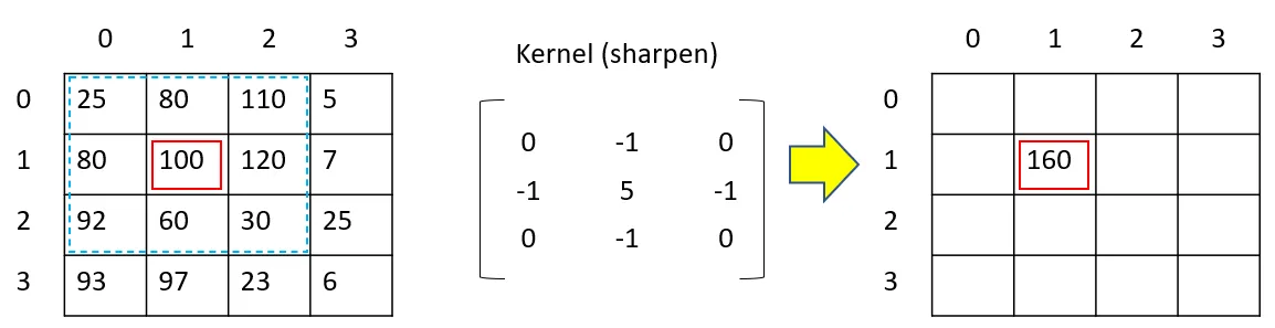
To elucidate this operation, consider a set of pixels from the image’s top-left corner. When applying the convolution kernel of size (2×2) to the pixel at position (1,1):
The filter evaluates values surrounding the target pixel, spanning from (x-1, y-1) to (x+1, y+1). These values are then multiplied by their respective elements in the kernel matrix. The results are summed up to produce the new pixel value.
This convolution is executed across the image, save for certain edge pixels. A question arises: How do we handle edge pixels, such as the one at (0,0)? There are several techniques to address this, including extending, wrapping, mirroring, or cropping the image (or occasionally the kernel). If this piques your curiosity, a detailed explanation is available here.
Kernels can produce varied effects depending on their values. Many of these filters are identifiable by specific names. For a visual illustration, refer to the Wikipedia article linked above.
In the following tasks, we implement convolutions using two approaches.
We provide a python script for testing your implementation. You can use the following commands to generate and print the input images. We also provide a canny edge detection implementation, which is a common image processing task that heavily relies on convolutions.
$ cd $REPO/conv

# Here is a Python testbench for your implementation in C++ (convolution.cpp)
# convolution.cpp contains the C++ code you will be updating.
# convolution.cpp will be compiled to a shared library similar previous tasks.
# conv_test.py expects a shared library called "convolution.so"

$ g++ -shared -o convolution.so -fPIC convolution.cpp
$ python3 conv_test.py

# Run Canny Edge Detection on F.jpg. This will output an image "F_gray.jpg".
$ python3 main.py --path ./F.jpg
Task 1: Tiled Convolutions
Convolution calculation can be tiled similar to matrix multiplication to improve data reuse and reduce memory traffic. The idea is to divide the image into smaller tiles and perform the convolution on these tiles. In this task, you are required to modify the implementation we provide in convolution.cpp to perform tiled convolutions. The following gif illustrates the concept of tiled convolutions.

Q11: Compare the performance for various tile sizes from 2x2,4x4,8x8,16x16 to the sequential convolution.
Task 2: Line buffer
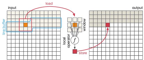
A special case of tiling can be employed where the tile size is 1xN. This is called a line buffer. The line buffer is a common optimization technique used in convolutional neural networks (CNNs) to improve data reuse and reduce memory traffic. The idea is to store a line of pixels from the image in a buffer and reuse it for multiple convolutions. Line buffers permit the flat array to be streamed in one row at a time and improves prefetching and caching. This is illustrated in Figure below. The height of the line buffer is dependent on the size of the filter. For example, a 3x3 filter would require a line buffer of height 3, while a 5x5 filter would require a line buffer of height 5. Implement line buffering and compare it to the tiled convolutions.
Q12: Compare the line buffer design with corresponding tile sizes from Q11.
Task 3: Convolution as a GEMM.
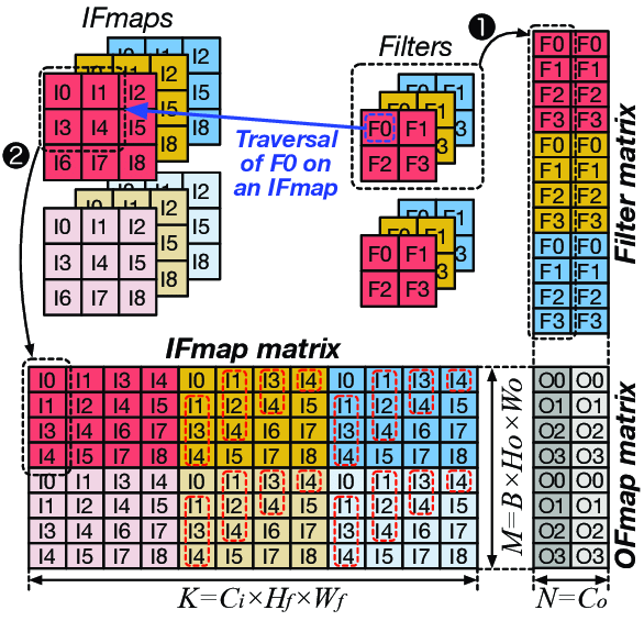
Finally, convolutions can be implemented as a gemm by preprocessing the input image. im2col is a common technique used to convert the image into a matrix. The idea is to extract patches from the image and store them as columns in a matrix. The size of the patches is determined by the kernel size. The resulting matrix is then multiplied with the flattened kernel matrix to produce the output image. This is illustrated in Figure below.
The illustration is for an rgb image; however in the assignment you are expected to implement only grayscale i.e., you can assume number of channels is always 1. Furthermore the illustration is for multiple filters (like in typical DNNs). Here we only have a single filter (which eliminates the need for a filter matrix).
-
You can assume the filter matrices are fixed and known at compiler time. You don’t have to measure the time taken for them; here we only use a single filter for any given invocation.
-
You can leverage the gemm implementation from Module 1. However, note that in module 1 you may tested with square matrices; here the matrix could be tall and narrow. Furthermore, the filter matrix does not need to be actually stored as a matrix as the filter values simply repeat. You can simply store the filter values in a small array and use it to multiply with the im2col matrix.
Your task is to implement im2col and compare the performance of convolution as a GEMM with the sequential convolution.
You may want to run your GEMM-based convolution through the provided Canny Edge Detection implementation to verify correctness.
Q13: How does the performance of convolution as a GEMM compare to the sequential convolution?
Grading
The assignment will be graded out of 150 points. The breakdown of points is as follows:
| Task | Points |
|---|---|
| GEMM | 30 |
| BCSR | 60 |
| CONV | 60 |