• Like the Fibonacci Sequence: \(f_0=0\), \(f_1=1\), \(f_n=f_{n-1}+f_{n-2}\).
• The last part of that, where the next term depends on previous ones is called a “recurrence relation”.

• We can say that we have a solution to the recurrence relation if we have a non-recursive way to express the terms.
• The initial conditions give the first term(s) of the sequence, before the recurrence part can take over.

• The terms of the sequence are \(1, 3, 5, 7, 9,\ldots\).
• A solution is \(a_n=2n-1\).

• A game where you have \(n\) disks of decreasing size stacked on a peg. Your job is to move the tower to another peg.
• You can only move one disk at a time, and cannot put a larger disk on a smaller one.
• For \(n=4\), winning the game looks like this:

  
  From Wikipedia's Tower_of_Hanoi_4.gif

• How many moves does it take to move \(n\) disks? Call this number \(H_n\).

procedure hanoi_move(n, from, to, other)
    if n=0:
        return
    hanoi_move(n-1, from, other, to)
    move one disk from the "from" peg to the "to" peg
    hanoi_move(n-1, other, to, from)

• Now we can see that we have the recurrence relation \(H_n=2H_{n-1}+1\). Our initial condition is \(H_1=1\).
• The values in the sequence are: 1, 3, 7, 15, 31, 63,…
• We can get a solution with a little algebra: \[\begin{align*} H_n &= 2H_{n-1} + 1\\ &= 4H_{n-2}+2+1 \\ &= 8H_{n-3}+4+2+1 \\ &\vdots\\ &= 2^{n-1}H_1+2^{n-2}+2^{n-3}+\cdots+4+2+1 \\ &= 2^{n-1}+2^{n-2}+2^{n-3}+\cdots+4+2+1 \\ &= 2^{n}-1\,. \end{align*}\]
• We could have also looked at the first terms of the sequence, guessed \(H_n=2^{n}-1\) and proved it by induction:

  Base case: For \(n=1\), it's true.

  Induction case: Assume for induction that \(H_{n-1}=2^{n-1}-1\). Then, \[\begin{align*} H_n &= 2H_{n-1} + 1\\ &= 2(2^{n-1}-1) + 1\\ &= 2^n-1\,.\quad ∎ \end{align*}\]

• Faster calculation, better idea of growth rate, etc.

• e.g. the logistic map, \(x_{n+1} = rx_n(1-x_n)\).
• I don't know of any functions that have behaviour like this as \(r\) increases:

  
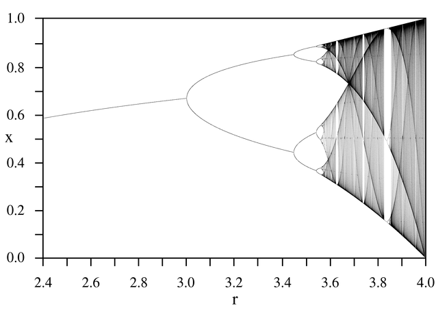
  From Wikimedia LogisticMap BifurcationDiagram.png

• If you really want to call these something, they're linear homogeneous recurrence relations of degree \(k\).
• Obviously, we need to give the \(k\) first terms as initial conditions.

• That will be true if \[r^n=a_n=c_{1}r^{n-1}+c_{2}r^{n-2}+\cdots +c_{k+1}r^{n-(k+1)} +c_{k}r^{n-k}\,.\]
• A little algebra gives us \[r^n-c_{1}r^{n-1}-c_{2}r^{n-2}-\cdots -c_{k+1}r^{n-(k+1)} -c_{k}r^{n-k}=0\\ r^k-c_{1}r^{k-1}-c_{2}r^{k-2}-\cdots -c_{k+1}r-c_{k}=0 \,.\]
• The second line there is the characteristic equation of this recurrence relation.
• Its solutions are the characteristic roots.

Theorem: Suppose we have a linear homogeneous recurrence relation \[a_n=c_{1}a_{n-1}+c_{2}a_{n-2}+\cdots +c_{k}a_{n-k}\,,\] and its characteristic equation, \[r^k-c_{1}r^{k-1}-c_{2}r^{k-2}-\cdots -c_{k+1}r-c_{k}=0\,.\] If the equation has \(k\) distinct roots, \(r_1,r_2,\ldots,r_k\), then \(\{a_n\}\) is a solution to the recurrence relation if and only if \[a_n=d_1r_1^n + d_2r_2^n+\cdots+d_k r_k^n\,,\] for some constants \(d_1,d_2,\ldots,d_k\).

Example: What is the solution to the recurrence relation \(a_n=2a_{n-1}+3a_{n-2}\), with \(a_0=3\) and \(a_1=5\)?

The characteristic equation for this recurrence is \(0=r^2-2r-3=(r-3)(r+1)\), which has roots \(r_1=3\) and \(r_2=-1\). Now we have a solution in the form \(a_n=d_1 3^n + d_2(-1)^n\), for some \(d_1\) and \(d_2\).

We can find the constants from the initial values we know: \[ a_0=d_1 3^0 + d_2(-1)^0 = d_1+d_2 =3\,,\\ a_1=d_1 3^1 + d_2(-1)^1=3d_1 - d_2=5\,. \] Adding these equations, we get \(4d_1=8\), so \(d_1=2\). And then from the first equation, we have \(d_2=1\).

Finally, we have a solution: \(a_n=2\cdot 3^n + (-1)^n\).

• We can calculate the first few terms, either with the recurrence or the solution: 3, 5, 19, 53, 163, 485.
• I got the same result both ways.

Example: We had a closed-form formula to calculate the Fibonacci numbers earlier. This theorem will find it: \(f_0=0\), \(f_1=1\), \(f_n=f_{n-1}+f_{n-2}\).

The characteristic equation is \(r^2-r-1=0\), which has roots \(r_1=\frac{1+\sqrt{5}}{2}\) and \(r_2=\frac{1-\sqrt{5}}{2}\). Thus we have a solution in the form \[f_n=d_1\left(\tfrac{1+\sqrt{5}}{2}\right)^n+d_2\left(\tfrac{1-\sqrt{5}}{2}\right)^n\,.\]

Again, we can use the initial conditions to solve for the constants: \[\begin{align*} f_0&=d_1+d_2=0\,,\\ f_1&=d_1\tfrac{1+\sqrt{5}}{2}+d_2\tfrac{1-\sqrt{5}}{2}=1\,. \end{align*}\]

Solving these equations, we get \(d_1=1/\sqrt{5}\) and \(d_2=-1/\sqrt{5}\). Thus we have \[f_n=\tfrac{1}{\sqrt{5}}\left(\tfrac{1+\sqrt{5}}{2}\right)^n-\tfrac{1}{\sqrt{5}}\left(\tfrac{1-\sqrt{5}}{2}\right)^n \,.\]

• … with distinct roots.
• And the related theorem in the text can handle characteristic equations with repeated roots.

• Suppose we ignore the non-linear part and just look at the homogeneous part: \[h_n=c_1h_{n-1} + c_2h_{n-2} + \cdots + c_kh_{n-k}\,.\]
• We can solve that and get a formula for \(\{h_n\}\).
• If we're lucky, we might be able to find a solution for \(\{a_n\}\) for some initial conditions, but maybe not the ones we're interested in

• We can use the previous theorem (or just guess-and-prove) that solutions to \(h_n=3h_{n-1}\) are in the form \(h_n=d\cdot 3^{n}\).
• If are willing to accept any initial conditions, we might be able to get a particular solution \(\{p_n\}\).
• We could guess that there might be a linear solution in the form \(p_n=cn+d\) for some constants \(c,d\).
• We would be right. There is such a solution iff for all \(n> 1\): \[\begin{align*} p_n &= 3p_{n-1} + 2n \\ cn+d&= 3(c(n-1)+d) + 2n \\ cn+d&= 3cn-3c+3d+2n \\ 0&=(2c+2)n+(2d-3c)\,. \end{align*}\] This is true for all \(n\) iff \(2c+2=0\) and \(2d-3c=0\). Solving these, we get \(c=-1\) and \(d=-3/2\).
• We have a solution to the recurrence: \(p_n=-n-3/2\).
• That isn't actually a useful solution: we're interested in \(a_1=3\) and that's not what \(p_1\) is. We have the wrong initial conditions.

Theorem: For a recurrence relation in the form \[a_n=c_1a_{n-1} + c_2a_{n-2} + \cdots + c_ka_{n-k} + F(n)\,,\] if we have a solution to the homogenous linear part \(\{h_n\}\) (as described above), and a particular solution \(\{p_n\}\), then all solutions to the recurrence are in the form \(\{h_n+p_n\}\).

Proof: Suppose we have any solution to the original recurrence: \(\{a_n\}\). We know that \(\{p_n\}\) is also a solution: \[ a_n=c_1a_{n-1} + c_2a_{n-2} + \cdots + c_ka_{n-k} + F(n)\\ p_n=c_1p_{n-1} + c_2p_{n-2} + \cdots + c_kp_{n-k} + F(n)\\ \]

Subtracting these, we get \[a_n-p_n=c_1(a_{n-1}-p_{n-1}) + c_2(a_{n-2}-p_{n-2})+ \cdots + c_k(a_{n-k}-p_{n-k})\] Thus, \(\{a_n-p_n\}\) is a solution to the homogenous part, \(\{h_n\}\).

So, any solution \(\{a_n\}\) is can be written in the form \(\{p_n+h_n\}\) for some solution to the homogenous recurrence.∎

• The above theorem tells us that all solutions to the recurrence look like \(a_n=d\cdot 3^{n}-n-3/2\).
• We just have to fill in \(d\): \[\begin{align*} a_1&=3 \\ d\cdot 3^{1}-1-3/2 &= 3 \\ d&= 11/6\,. \end{align*}\]
• We finally have \(a_n=11/6\cdot 3^{n}-n-3/2\).

• The homogeneous part of this is \(h_n=2h_{n-1}\). We could guess, but let's use the theorem.
• The characteristic equation for this recurrence is \(r-2=0\) which has solution \(r=2\). Thus, solutions are in the form \(h_n=d\cdot2^n\).
• For a particular solution guess that \(p_n=c\cdot 3^n\) for some \(c\). We can confirm the guess by finding a constant \(c\). To do this, we substituting into the recurrence: \[\begin{align*} p_n &= 2p_{n-1}+3^n\\ c\cdot 3^n &= 2(c\cdot 3^{n-1})+3^n\\ c(3^n-2\cdot 3^{n-1}) &= 3^n\\ c(3-2) &= 3^n/3^{n-1} \\ c&=3\,. \end{align*}\]
• We have a particular solution (for no particular initial conditions) of \(p_n=3^{n+1}\).
• Now we can satisfy \(a_n\) for our initial condition since all solutions to \(\{a_n\}\) are in the form \[\begin{align*} a_n &= d2^n + 3^{n+1}\\ 5=a_1 &= d2^1 + 3^2\\ 5 &= 2d+3\\ d&=2\,. \end{align*}\]
• So, \(a_n=2^{n+1}+ 3^{n+1}\).

• The homogeneous part has characteristic equation \(r^2-5r-6=0\), so roots \(r_1=6,r_2=-1\).
• So, solutions are in the form \(h_n=d_1 6^n+d_2 (-1)^n\).
• For a particular solution, we should find something in the form \(p_n=c\cdot 7^n\): \[\begin{align*} p_n = c\cdot 7^n &= 5c\cdot 7^{n-1}+6c\cdot 7^{n-2}+7^n \\ c\cdot 7^2 &= 5c\cdot 7^1+6c\cdot 7^0+7^2 \\ 0 &= 49/8\,. \end{align*}\]
• So we have \(p_n=\frac{49}{8}\cdot 7^n\).
• From the theorem, \[a_n=d_1 6^n+d_2 (-1)^n+\tfrac{49}{8}\cdot 7^n\,.\]
• Substituting \(a_0\) and \(a_1\), we get \[ 1=d_1+d_2+\tfrac{49}{8} \text{ and } 6=6d_1-d_2+\tfrac{343}{8}\,,\\ d_1=-6 \text{ and } d_2=\tfrac{7}{8}\,. \]
• Thus we have a solution: \[a_n= -6\cdot 6^n-\tfrac{7}{8}\cdot (-1)^n+\tfrac{49}{8}\cdot 7^n = \tfrac{1}{8}\left(-8\cdot 6^{n+1} - 7(-1)^n + 7^{n+2}\right) \,.\]
• I definitely wouldn't have come up with that without the theorem to help.

• That is, they split the problem into pieces (divide), and recurse on those pieces to solve the problem (conquer).

• Binary search: takes \(O(1)\) time in the recursive step, and recurses on half the list. Its running time is \(f(n)=f(n/2)+1\).
• Mergesort: takes \(O(n)\) time in the recursive step, and recurses on both halves of the list. Its running time is \(f(n)=2f(n/2)+n\).
• We stated running times for these, but only vaguely discussed why.

Theorem: (Master Theorem) For an increasing function \(f\) with the recurrence relation \[f(n)=af(n/b)+cn^d\,,\] with \(a\ge 1\), \(b>1\) an integer, \(c>0\), \(d\ge 0\), then \[ f(n) \text{ is } \begin{cases} O(n^d) & \text{if } a<b^d\,,\\ O(n^d\log n) & \text{if } a=b^d\,,\\ O(n^{log_b a}) & \text{if } a>b^d\,,\\ \end{cases} \]

Example: The text describes an algorithm to find the closest two pair in a set of \((x,y)\) points. The naïve would be to take every pair of points (\(C(n,2)\) of them), calculate the distance, and remember the smallest. That is \(O(n^2)\).

The algorithm starts by sorting the points by their \(x\) coordinate (\(O(n\log n)\)). The problem is then split in half and solved recursively. Finding the final solution from that takes \(7n\) comparisons. That gives a recurrence relation of \(f(n)=2f(n/2)+7n\).

Now, \(a=2,b=2,c=7,d=1\). Again, \(a=b^d\), so the algorithm is \(O(n^d\log n)=O(n\log n)\).

Example: Suppose we write a recursive algorithm to find the smallest element in a list

procedure smallest(list, start, end)
    if start ≥ end-1
        return list[start]
    else
        mid = ⌊(start+end)/2⌋
        small1 = smallest(list, start, mid)
        small2 = smallest(list, mid+1, end)
        return smallest of small1 and small2

Now we have \(a=2,b=2,c=2,d=0\) and \(a>b^d\). Thus the running time is \(O(n^{\log_2 2})=O(n)\).

That is, the divide-and-conquer strategy didn't gain us anything over the obvious left-to-right version of this algorithm.

Example: Suppose you come up with an algorithm with this general format:

procedure example(n)
    if n ≤ 1
        return
    else
        a = example(n/2)
        b = example(n/2)
        combine a and b using n2 steps

The running time of this algorithm is \(f(n)=2f(n/2) + n^2\).

For the Master Theorem, we have \(a=2,b=2,c=1,d=2\) and \(a<b^d\). Thus the running time is \(O(n^2)\).

So for large-enough \(d\), the recursion work doesn't matter and the recursive-step work dominates.