Although not obvious from Equation 4.1, the discrete implementation of the nonlinear anisotropic diffusion filter is straightforward. Three key ideas help map the problem from the continuous domain to the discrete domain:
Using these ideas, a 1D derivation for the filter will be described. The derivation will then be generalized to the 2D and 3D cases.
In one dimension, the gradient and divergence expressions in Equation 4.1 reduce to derivatives:

Substituting discrete approximations for the derivatives and introducing the flow functions we get:
 and
and  are functions of
  ,
,
 , and
, and  ; the notation has been dropped for simplicity.
 and
and  are easily computed by substituting
the discrete approximation of the gradient into
Equation 4.2:
are easily computed by substituting
the discrete approximation of the gradient into
Equation 4.2:

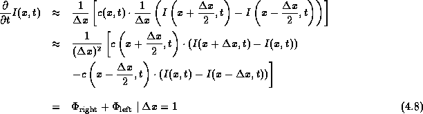
Equation 4.8 indicates that, for each iteration, the value of each element in a 1D array changes according to the flow contributed from its nearest neighbors. Figure 4.3 represents this concept graphically.
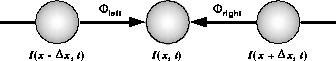
Figure 4.3: Visualization of 1D diffusion
between elements in an array.  is modified by the flow
contributions, and .
is modified by the flow
contributions, and .
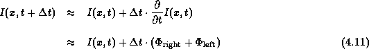
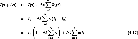
An expression for the discrete implementation of the 1D diffusion filter can be derived by determining the element values after each iteration:
The iteration scheme expressed in Equation 4.11 is
stable as long as  is sufficiently small. Bounds for
are computed in Section 4.3.4.
is sufficiently small. Bounds for
are computed in Section 4.3.4.
Note that the scheme is nonconvergent. Nordström provides a convergent version of the process he calls biased anisotropic diffusion [34]:

where  is the initial array before filtering.
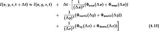
The 1D discrete formulation of the diffusion process is easily extended to the 2D case:
The filtering process consists of updating each pixel in the image by an amount equal to the flow contributed by its four nearest neighbors:

As with the 1D case, the 2D process can be represented graphically
(see Figure 4.4). Eight nearest neighbors can be used
if the flow contribution of the diagonal neighbors is scaled according
to their relative distance,  , from the pixel of interest:
Anisotropic images can be handled similarly. The 3D formulation that follows assumes anisotropicy.
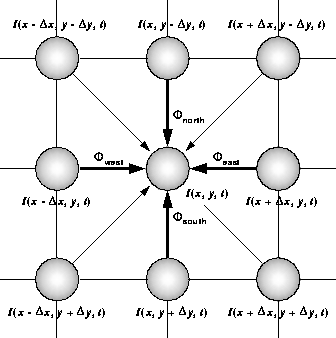
Figure 4.4: Visualization of 2D diffusion
among pixels in an image.  is modified by the flow
contributions,
is modified by the flow
contributions,  .
.
The discrete formulation of the 3D nonlinear anisotropic diffusion filter can be extrapolated from the 2D description. The 3D filter, utilizing six nearest neighbors, is expressed as:
where ,  , and
, and  are relative
distances between
are relative
distances between  and its nearest neighbors in the
,
and its nearest neighbors in the
,  , and
, and  dimensions respectively. This expression
assumes volume anisotropicy and can be extended to include 26 nearest
neighbors in a similar manner to the 2D case. Again, the functional
notation has been dropped from the flow functions for clarity.
dimensions respectively. This expression
assumes volume anisotropicy and can be extended to include 26 nearest
neighbors in a similar manner to the 2D case. Again, the functional
notation has been dropped from the flow functions for clarity.
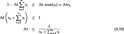
The discrete implementation of the nonlinear anisotropic diffusion filter is a numerical integration of a partial differential equation. Methods for analyzing the stability of numerical integrations can be found in many numerical analysis texts (see [42]).
Gerig et al. use a simple analysis to find bounds for the diffusion filter
integration constant, [17]. The analysis is
repeated here for completeness.
must be in the range,  , where
  is a
positive real number. The nearer is to zero, the closer
the integration approximates the continuous case. However, many
iteration steps would be required by the filter.
is a
positive real number. The nearer is to zero, the closer
the integration approximates the continuous case. However, many
iteration steps would be required by the filter.
The upper bound, , can be determined from the discrete
formulation of the diffusion process (spatial indices have been
dropped for clarity):
where the subscript,  , refers to the nearest
neighbors of
, refers to the nearest
neighbors of  . Data isotropicy has been assumed.
In order for the process described by
Equation 4.17 to be stable, the weight of the
central intensity, , must be greater than or equal to the
maximum weight of the neighborhood intensities,  :
:
By setting  in the diffusion functions from
equations 4.3 and 4.4 to infinity, the
diffusion coefficients,
in the diffusion functions from
equations 4.3 and 4.4 to infinity, the
diffusion coefficients,  , are maximized and equal to unity,
independent of gradient:
, are maximized and equal to unity,
independent of gradient:
Equation 4.19 assumes that the nearest neighbors are equidistant. The larger distance for diagonal neighbors in 2D and 3D data sets and the differing distances in anisotropic data sets are easily accounted for by adding a relative distance factor:

where  is the relative distance between neighbor,
  ,
and the central node.
,
and the central node.  for the four nearest neighbors
in images,
for the four nearest neighbors
in images,  for diagonal neighbors, and
 for the corners of neighborhood cubes in
volumes.
for the corners of neighborhood cubes in
volumes.
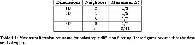
The bounds for for filters operating on isotropic data
sets are listed in Table 4.1.